Euler Examples

Search

Minimal Distances in the Plane

by Alain Busser

Preliminary remark

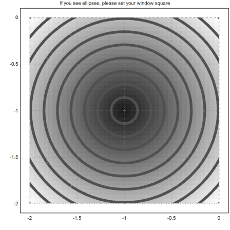
The function which, to a point M in the plane, assigns the distance AM between a fixed point A and M, has rather simple level lines: circles centered in A.

>A=[-1,-1];
>function d1(x,y):=sqrt((x-A[1])^2+(y-A[2])^2)
>fcontour("d1",xmin=-2,xmax=0,ymin=-2,ymax=0,hue=1, ...
 title="If you see ellipses, please set your window square"):

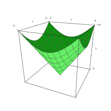
and the graph is rather simple too: the upper part of a cone:

>plot3d("d1",xmin=-2,xmax=0,ymin=-2,ymax=0):

Of course the minimum 0 is attained in A.

Two points

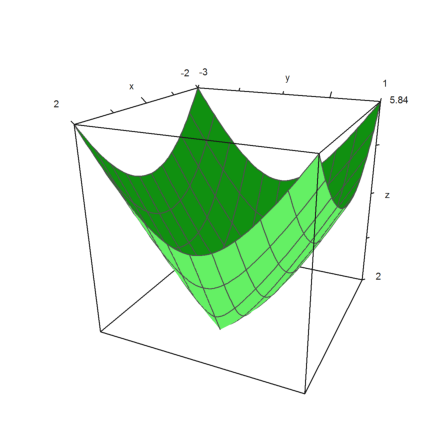
Now we look at the function MA+MB where A and B are two points (fixed). It is a "well-known fact" that the level curves are ellipses, the focal points being A and B; except for the minimum AB which is constant on the segment [AB]:

>B=[1,-1];
>function d2(x,y):=d1(x,y)+sqrt((x-B[1])^2+(y-B[2])^2)
>fcontour("d2",xmin=-2,xmax=2,ymin=-3,ymax=1,hue=1):

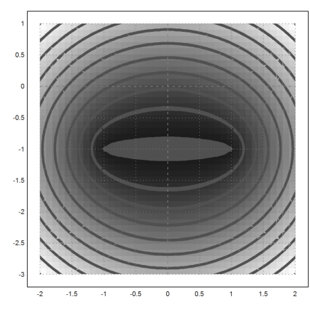
The graph is more interesting:

>plot3d("d2",xmin=-2,xmax=2,ymin=-3,ymax=1):

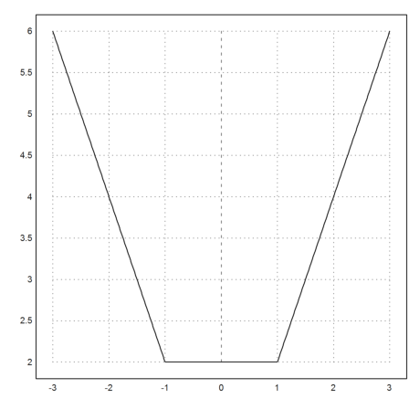
The restriction to line (AB) is more famous:

>plot2d("abs(x+1)+abs(x-1)",xmin=-3,xmax=3):

Three points

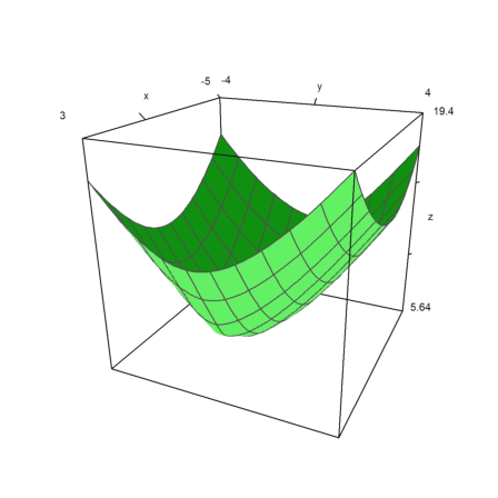
Now things are less simple: It is a little less well-known that MA+MB+MC attains its minimum at one point of the plane but to determine it is less simple:

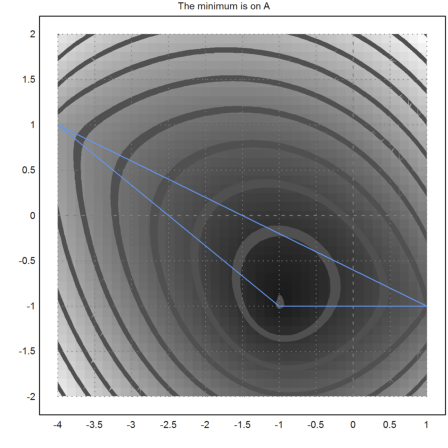
1) If one of the angles of the triangle ABC is more than 120° (say in A), then the minimum is attained at this very point (say AB+AC).

Example:

>C=[-4,1];
>function d3(x,y):=d2(x,y)+sqrt((x-C[1])^2+(y-C[2])^2)
>plot3d("d3",xmin=-5,xmax=3,ymin=-4,ymax=4);
>insimg;

>fcontour("d3",xmin=-4,xmax=1,ymin=-2,ymax=2,hue=1,title="The minimum is on A");
>P=(A_B_C_A)'; plot2d(P[1],P[2],add=1,color=12);
>insimg;

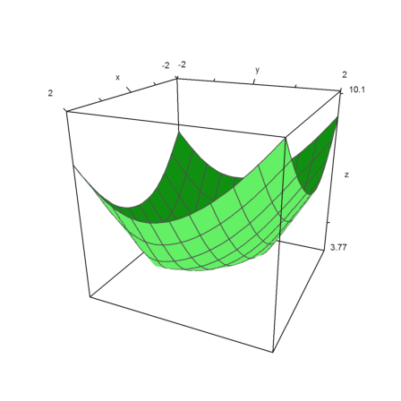
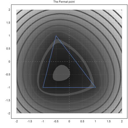
2) But if all the angles of triangle ABC are less than 120°, the minimum is on a point F in the interior of the triangle, which is the only point which sees the sides of ABC with the same angles (then 120° each):

>C=[-0.5,1];
>plot3d("d3",xmin=-2,xmax=2,ymin=-2,ymax=2):

>fcontour("d3",xmin=-2,xmax=2,ymin=-2,ymax=2,hue=1,title="The Fermat point");
>P=(A_B_C_A)'; plot2d(P[1],P[2],add=1,color=12);
>insimg;

It is an interesting activity to realize the above figure with a geometry software; for example, I know a soft written in Java which has a "contour lines" instruction...

All of this above have been discovered by a french judge called Pierre de Fermat; he wrote letters to other dilettants like the priest Marin Mersenne and Blaise Pascal who worked at the income taxes. So the unique point F such that FA+FB+FC is minimal, is called the Fermat point of the triangle. But it seems that a few years before, the italian Torriccelli had found this point before Fermat did! Anyway the tradition is to note this point F...

Four points

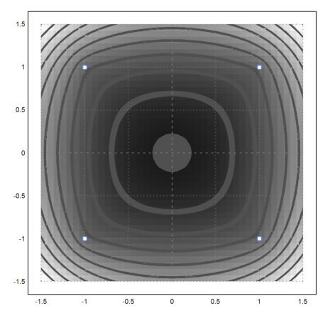
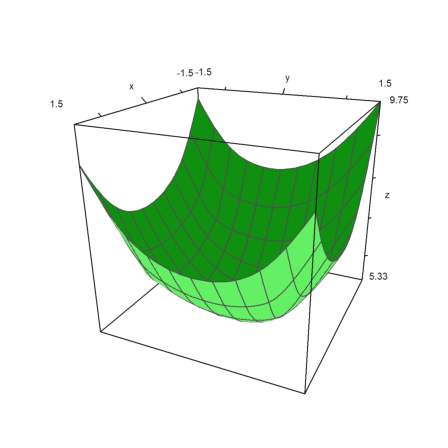
The next step is to add a 4th point D and try and minimize MA+MB+MC+MD; say that you are a cable TV operator and want to find in which field you must put your antenna so that you can feed four villages and use as little cable length as possible!

>D=[1,1];
>function d4(x,y):=d3(x,y)+sqrt((x-D[1])^2+(y-D[2])^2)
>plot3d("d4",xmin=-1.5,xmax=1.5,ymin=-1.5,ymax=1.5):

>fcontour("d4",xmin=-1.5,xmax=1.5,ymin=-1.5,ymax=1.5,hue=1);
>P=(A_B_C_D)'; plot2d(P[1],P[2],points=1,add=1,color=12);
>insimg;

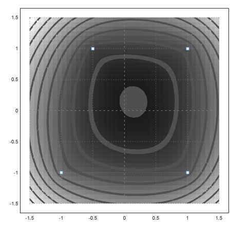
There is still a minimum and it is attained at none of the vertices A, B, C nor D:

>function f(x):=d4(x[1],x[2])
>neldermin("f",[0.2,0.2])

[0.142858,  0.142857]

It seems that in this case, the coordinates of the optimal point are rational or near-rational...

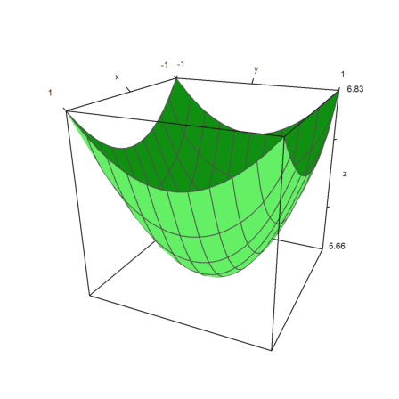
Now ABCD is a square we expect that the optimal point will be the center of ABCD:

>C=[-1,1];
>plot3d("d4",xmin=-1,xmax=1,ymin=-1,ymax=1):

>fcontour("d4",xmin=-1.5,xmax=1.5,ymin=-1.5,ymax=1.5,hue=1);
>P=(A_B_C_D)'; plot2d(P[1],P[2],add=1,color=12,points=1);
>insimg;

Examples